畳み込み層を実装してみる
この辺の続き。
畳み込み層とプーリング層、ひいては CNN をしてみる。
前回の im2col 連中を、バッチサイズ/チャンネルとか踏まえて再実装。
超長いので、今回はここから続きを読むリンク…。
import numpy as np
import matplotlib.pyplot as plt
%matplotlib inline


def im2col(images, filter_height, filter_width, out_height, out_width, stride, padding):
    """im2col 実装

    Args:
        images (np.Array): バッチ-チャンネル-画像の縦軸-画像の横軸 の4次元テンソル
        filter_height (integer): フィルタの高さ
        filter_width (integer): フィルタの幅
        out_height (integer): 出力見込みの画像高さ
        out_width (integer): 出力見込みの画像幅
        stride (integer): フィルタを適用するピクセル幅
        padding (integer): 画像の周囲に埋め込む 0 パディング幅
    """
    batch_size, channels, img_hight, img_width = images.shape
    img_padding = np.pad(images, [(0,0), (0,0), (padding, padding), (padding, padding)], "constant")
    cols = np.zeros((batch_size, channels, filter_height, filter_width, out_height, out_width))
    for h in range(filter_height):
        h_lim = h + stride*out_height
        for w in range(filter_width):
            w_lim = w + stride*out_width
            cols[:, :, h, w, :, :] = img_padding[:, :, h:h_lim:stride, w:w_lim:stride]
    cols = cols.transpose(1, 2, 3, 0, 4, 5).reshape(channels*filter_height*filter_width, batch_size*out_height*out_width)
    return cols

def col2im(cols, img_shape, filter_height, filter_width, out_height, out_width, stride, padding):
    """col2im, im2col の逆実装

    Args:
        cols (np.Array): im2col されたデータ
        img_shape (Array): バッチサイズ,チャンネル数,画像高さ,画像幅の配列
        filter_height (integer): フィルタの高さ
        filter_width (integer): フィルタの幅
        out_height (integer): 出力予定の画像高さ
        out_width (integer): 出力予定の画像幅
        stride (integer): フィルタ適用幅
        padding (integer): 画像周囲に埋め込まれる 0 パディング幅
    """
    batch_size, channels, img_hight, img_width = img_shape
    cols = cols.reshape(channels, filter_height, filter_width, batch_size, out_height, out_width, ).transpose(3, 0, 1, 2, 4, 5)
    images = np.zeros((batch_size, channels, img_hight+2*padding+stride-1, img_width+2*padding+stride-1))
    for h in range(filter_height):
        h_lim = h + stride*out_height
        for w in range(filter_width):
            w_lim = w + stride*out_width
            images[:, :, h:h_lim:stride, w:w_lim:stride] += cols[:, :, h, w, :, :]
    return images[:, :, padding:img_hight+padding, padding:img_width+padding]
で、NN でおなじみの活性関数軍
def relu_func(x):
    return np.where(x <= 0, 0, x)

def relu_func_dash(y, t):
    return y * np.where(t <= 0, 0, 1)

def soft_max(u):
    return np.exp(u) / np.sum(np.exp(u), axis=1).reshape(-1, 1)

def soft_max_dash(y, t):
    return y - t


# あと無駄かもしれんけど
class ILayer:
    def forward(self, x):
        pass
    def backward(self, grad_y):
        pass
    def update(self):
        pass
インターフェース置いといた理由は、のちにこれ配列にできんじゃない?って思ったから。
配列にしてしまえば層増やし放題なんで…。
畳み込み層の実装
eta = 0.01  # 学習係数
wb_width = 0.1  # 重みとバイアスの広がり具合


class ConvLayer(ILayer):
    """畳み込み層実装"""

    def __init__(self, x_channel, x_height, x_width, filter_num, filter_height, filter_width, stride, padding):
        """これから処理する画像の情報、フィルタ設定などを指定する。

        Args:
            x_channel (integer): チャンネル数
            x_height (integer): 画像の高さ
            x_width (integer): 画像の幅
            filter_num (integer): フィルタ個数
            filter_height (integer): フィルタの高さ
            filter_width (integer): フィルタの幅
            stride (integer): フィルタを適用するステップ数
            padding (integer): パディング幅
        """
        self.params = (x_channel, x_height, x_width, filter_num, filter_height, filter_width, stride, padding)

        # ランダムな重みとバイアス
        self.w = wb_width * np.random.randn(filter_num, x_channel, filter_height, filter_width)
        self.b = wb_width * np.random.randn(1, filter_num)

        # y = この層の出力行列サイズパラメータ
        self.y_ch = filter_num  # 出力チャンネル数=フィルタ数
        self.y_h = (x_height - filter_height + 2*padding) // stride + 1
        self.y_w = (x_width - filter_width + 2*padding) // stride + 1

        # AdaGrad用変数
        self.h_w = np.zeros((filter_num, x_channel, filter_height, filter_width)) + 1e-8
        self.h_b = np.zeros((1, filter_num)) + 1e-8

    def forward(self, x):
        """順伝播"""
        batch_num = x.shape[0]
        x_channel, x_height, x_width, filter_num, filter_height, filter_width, stride, padding = self.params
        y_ch, y_h, y_w = self.y_ch, self.y_h, self.y_w

        # 入力画像とフィルタを行列に変換
        self.cols = im2col(x, filter_height, filter_width, y_h, y_w, stride, padding)
        self.w_col = self.w.reshape(filter_num, x_channel*filter_height*filter_width)

        # 重みとバイアスを設定して
        u = np.dot(self.w_col, self.cols).T + self.b
        self.u = u.reshape(batch_num, y_h, y_w, y_ch).transpose(0, 3, 1, 2)

        # relu 関数を適用
        self.y = relu_func(self.u)
        return self.y

    def backward(self, grad_y):
        """逆伝播関数"""
        batch_num = grad_y.shape[0]
        x_channel, x_height, x_width, filter_num, filter_height, filter_width, stride, padding = self.params
        y_ch, y_h, y_w = self.y_ch, self.y_h, self.y_w

        # relu の微分更新式を適用
        delta = relu_func_dash(grad_y, self.u)
        delta = delta.transpose(0,2,3,1).reshape(batch_num*y_h*y_w, y_ch)

        # フィルタとバイアスの勾配
        grad_w = np.dot(self.cols, delta)
        self.grad_w = grad_w.T.reshape(filter_num, x_channel, filter_height, filter_width)
        self.grad_b = np.sum(delta, axis=0)

        # 入力の勾配
        grad_cols = np.dot(delta, self.w_col)
        x_shape = (batch_num, x_channel, x_height, x_width)
        self.grad_x = col2im(grad_cols.T, x_shape, filter_height, filter_width, y_h, y_w, stride, padding)
        return self.grad_x

    def update(self):
        # AdaGrad で勾配更新に制限をかける
        self.h_w += self.grad_w * self.grad_w
        self.w -= eta / np.sqrt(self.h_w) * self.grad_w
        self.h_b += self.grad_b * self.grad_b
        self.b -= eta / np.sqrt(self.h_b) * self.grad_b
ニューロン程変化するものでもない気がしたのでべた書き。
コンポーリューションというとあれだけど、順伝播時は入力画像に重みづけとバイアス(この二つがフィルタ扱い)をかけて、ReLU に食わせてるだけ。
活性関数を利用するので、当然逆伝播でも微分してきます。
Pooling 層
こいつは何してるかというと、画像をいくつかの部分部分に分割してその最大値を取ってくるという処理をしている。
なんでそんな処理するのか?って考えると、絵とか画像って狭い範囲を見ると、特定のドットの色は周囲のドットの色に影響を受けてるという論理で、「画像の部分部分の最大値を拾っておけば特徴ってとれるよね!」という論理に基づいてる。
こいつに学習はない…というかどう考えても固定フィルタなので…
class PoolingLayer(ILayer):
    """プーリング層実装: フィルタサイズ指定で Max プーリングを実行する。平たく言うと、画像の部分部分で最大値を引っこ抜いて縮小する"""

    def __init__(self, x_channel, x_height, x_width, pooling_size, padding):
        """これから処理する画像の情報、フィルタ設定などを指定する。

        Args:
            x_channel ([type]): [description]
            x_height ([type]): [description]
            x_width ([type]): [description]
            pooling_size ([type]): [description]
            padding ([type]): [description]
        """
        self.params = (x_channel, x_height, x_width, pooling_size, padding)

        # Output tensor params.
        self.y_ch = x_channel
        self.y_h = x_height // pooling_size if x_height%pooling_size == 0 else x_height // pooling_size + 1
        self.y_w = x_width // pooling_size if x_width%pooling_size == 0 else x_width // pooling_size + 1

    def forward(self, x):
        n_bt = x.shape[0]
        x_channel, x_height, x_width, pooling_size, padding = self.params
        y_ch, y_h, y_w = self.y_ch, self.y_h, self.y_w
        # Converting
        cols = im2col(x, pooling_size, pooling_size, y_h, y_w, pooling_size, padding)
        cols = cols.T.reshape(n_bt*y_h*y_w*x_channel, pooling_size*pooling_size)
        # Exec Max pooling
        y = np.max(cols, axis=1)
        self.y = y.reshape(n_bt, y_h, y_w, x_channel).transpose(0, 3, 1, 2)
        # Caching max indexes
        self.max_index = np.argmax(cols, axis=1)

        return self.y

    def backward(self, grad_y):
        n_bt = grad_y.shape[0]
        x_channel, x_height, x_width, pooling_size, padding = self.params
        y_ch, y_h, y_w = self.y_ch, self.y_h, self.y_w

        grad_y = grad_y.transpose(0, 2, 3, 1)

        # 行列を作成し、各列の最大値であった要素にのみ出力の勾配を入れる
        grad_cols = np.zeros((pooling_size*pooling_size, grad_y.size))
        grad_cols[self.max_index.reshape(-1), np.arange(grad_y.size)] = grad_y.reshape(-1)
        grad_cols = grad_cols.reshape(pooling_size, pooling_size, n_bt, y_h, y_w, y_ch)
        grad_cols = grad_cols.transpose(5,0,1,2,3,4)
        grad_cols = grad_cols.reshape( y_ch*pooling_size*pooling_size, n_bt*y_h*y_w)

        # 入力の勾配
        x_shape = (n_bt, x_channel, x_height, x_width)
        self.grad_x = col2im(grad_cols, x_shape, pooling_size, pooling_size, y_h, y_w, pooling_size, padding)

        return self.grad_x
で、その先の NN は前回までのニューラルネット実装を拝借。
AdaGrad/ReLU/SoftMax で処理するよーコピペできるって楽
class Neuron(ILayer):
    def __init__(self, n_upper, n, activation_function, differential_function):
        self.w = wb_width * np.random.randn(n_upper, n) # ランダムなのが確立勾配法
        self.b = wb_width * np.random.randn(n)
        self.grad_w = np.zeros((n_upper, n))
        self.grad_b = np.zeros((n))
        self.activation_function = activation_function
        self.differential_function = differential_function

    def update(self):
        self.w -= eta * self.grad_w
        self.b -= eta * self.grad_b

    def forward(self, x):
        self.x = x
        u = x.dot(self.w) + self.b
        self.y = self.activation_function(u)
        return self.y

    def backward(self, t):
        delta = self.differential_function(self.y, t)
        self.grad_w = self.x.T.dot(delta)
        self.grad_b = np.sum(delta, axis=0)
        self.grad_x = delta.dot(self.w.T)
        return self.grad_x


class AdaNeuron(Neuron):
    def __init__(self, n_upper, n, activation_function, differential_function):
        super().__init__(n_upper, n, activation_function, differential_function)
        self.h_w = np.zeros((n_upper, n)) + 1e-8
        self.h_b = np.zeros((n)) + 1e-8

    def update(self):
        # AdaGrad で更新にリミットを設ける。
        self.h_w += (self.grad_w * self.grad_w)
        self.h_b += (self.grad_b * self.grad_b)
        self.w -= eta / np.sqrt(self.h_w) * self.grad_w
        self.b -= eta / np.sqrt(self.h_b) * self.grad_b


class Output(AdaNeuron):
    pass


class Middle(AdaNeuron):
    def backward(self, grad_y):
        delta = self.differential_function(grad_y, self.y)
        self.grad_w = self.x.T.dot(delta)
        self.grad_b = delta.sum(axis = 0)
        self.grad_x = delta.dot(self.w.T)
        return self.grad_x
テストする画像
scikitlearn には minist データセットというやつらがいる。
こいつらは要するに手書き数字のデータセット
from sklearn import datasets
from sklearn.model_selection import train_test_split

digits_data = datasets.load_digits()
input_data = digits_data.data
correct = digits_data.target
n_data = len(correct)

# 画像の表示
plt.imshow(digits_data.data[0].reshape(8, 8), cmap="gray")
plt.show()

こんな感じの 8x8 ピクセル画像。
検証用にさっさとデータセット分割する
# 標準化
def standardize(x):
    av = np.average(x)
    std = np.std(x)
    return (x - av) / std
input_data = standardize(input_data)


# 回答データを One-Hot に変換
correct_data = np.zeros((n_data, 10))
for i in range(n_data):
    correct_data[i, correct[i]] = 1.0


# 学習データとテストデータの分離
X_train, X_test, y_train, y_test = train_test_split(input_data, correct_data, random_state=0)

n_train = X_train.shape[0]  # 訓練データのサンプル数
n_test = X_test.shape[0]    # テストデータのサンプル数
いざ、CNN を構築しようか
# 白黒で 8x8 ピクセル
img_height = 8
img_width = 8
img_channel = 1

# 学習セットサイズ
epoch = 50
batch_size = 8

# デバッグ出力設定
interval = 10
n_sample = 200


# 畳み込み層
conv_layer = ConvLayer(
    x_channel=img_channel,
    x_height=img_height,
    x_width=img_width,
    filter_num=10,
    filter_height=3,
    filter_width=3,
    stride=1,
    padding=1
)

# プーリング層
pooling_layer = PoolingLayer(
    x_channel=conv_layer.y_ch,
    x_height=conv_layer.y_h,
    x_width=conv_layer.y_w,
    pooling_size=2,
    padding=0
)

# 中間層と出力層
polling_result = pooling_layer.y_ch * pooling_layer.y_h * pooling_layer.y_w
# 中間層は 100 ニューロン
middle_layer = Middle(polling_result, 100, relu_func, relu_func_dash)
# 結果は 0-9 の 10 通りなので 10 ニューロン
output_layer = Output(100, 10, soft_max, soft_max_dash)


def forwardpropagation(x):
    """順伝播"""
    batch_size = x.shape[0]

    images = x.reshape(batch_size, img_channel, img_height, img_width)
    y = pooling_layer.forward(conv_layer.forward(images))

    fc_input = y.reshape(batch_size, -1)
    output_layer.forward(middle_layer.forward(fc_input))


def backpropagation(t):
    """逆伝播"""
    batch_size = t.shape[0]
    grad_x = middle_layer.backward(output_layer.backward(t))

    grad_img = grad_x.reshape(batch_size, pooling_layer.y_ch, pooling_layer.y_h, pooling_layer.y_w)
    conv_layer.backward(pooling_layer.backward(grad_img))


def update_layers():
    """重みとバイアスの更新"""
    conv_layer.update()
    middle_layer.update()
    output_layer.update()


def calc_error(t, batch_size):
    """エントロピー誤差を計算"""
    return -np.sum(t * np.log(output_layer.y + 1e-7)) / batch_size


def forward_sample(inp, correct, n_sample):
    """サンプルを順伝播"""
    index_rand = np.arange(len(correct))
    np.random.shuffle(index_rand)
    index_rand = index_rand[:n_sample]
    x = inp[index_rand, :]
    t = correct[index_rand, :]
    forwardpropagation(x)
    return x, t
後は呼び出すだけでござる
# for debug.
train_error_x = []
train_error_y = []
test_error_x = []
test_error_y = []

n_batch = n_train // batch_size
for i in range(epoch):

    # Calc current errors.
    x, t = forward_sample(X_train, y_train, n_sample)
    error_train = calc_error(t, n_sample)
    x, t = forward_sample(X_test, y_test, n_sample)
    error_test = calc_error(t, n_sample)

    # Save errors.
    train_error_x.append(i)
    train_error_y.append(error_train)
    test_error_x.append(i)
    test_error_y.append(error_test)

    # DEBUG display
    if i%interval == 0:
        print(f"Epoch: {i}/{epoch}, Error_train: {error_train}, Error_test: {error_test}")

    # Learning
    index_rand = np.arange(n_train)
    np.random.shuffle(index_rand)
    for j in range(n_batch):
        mb_index = index_rand[j*batch_size : (j+1)*batch_size]
        x = X_train[mb_index, :]
        t = y_train[mb_index, :]

        forwardpropagation(x)
        backpropagation(t)
        update_layers()

# 誤差の推移表示
plt.plot(train_error_x, train_error_y, label="Train")
plt.plot(test_error_x, test_error_y, label="Test")
plt.legend()

plt.xlabel("Epochs")
plt.ylabel("Error")

plt.show()
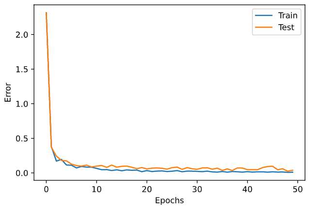
画像判定はかなり正確にできたっぽい。
x, t = forward_sample(X_train, y_train, n_train)
count_train = np.sum(np.argmax(output_layer.y, axis=1) == np.argmax(t, axis=1))
x, t = forward_sample(X_test, y_test, n_test)
count_test = np.sum(np.argmax(output_layer.y, axis=1) == np.argmax(t, axis=1))

print(f"Accuracy Train: {count_train/n_train*100} %, Test: {count_test/n_test*100} %")
ということで、テストデータと検証データで正解率を見てみると
Accuracy Train: 100.0 % Accuracy Test: 98.88888888888889 %
ひゃっほい。
前処理で、きっちり数字部分の画像切り抜いて、8x8 画像にして食わせばこのくらいの精度で判定してくれるってことで。