RNN で時系列データの予測をやってみる
この辺の続き
要するに次の値を予測してもらうという NN ですな
まずは結果から
正弦波にノイズを与えたデータが学習データ青で、先頭 10 件だけはそのまま、11 件目以降を 10 件づつ与えたデータから予測させて作ったグラフが黄色である。
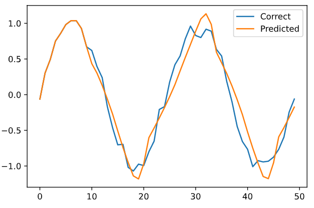
ん、まぁなんとなく正しそうな予感はする。
株価みたいな線形データならやれるだろうか…取り込めるデータは1系統なので、特定銘柄特化でならなりそうな気はするが…。
で、ソース。
学習データソースはこんな感じ。
import numpy as np
import matplotlib.pyplot as plt

%matplotlib inline

# ダミー学習データ(X軸範囲)
sin_x = np.linspace(-2 * np.pi, 2 * np.pi)
# ノイズを載せる
sin_y = np.sin(sin_x) + 0.1 * np.random.randn(len(sin_x))
これを学習するにあたってデータ形状変換
n_time = 10
n_in   = 1   # 入力層ニューロン数
n_mid  = 20  # 中間層ニューロン数
n_out  = 1   # 出力層ニューロン数

# 学習データ
n_sample     = len(sin_x) - n_time
input_data   = np.zeros((n_sample, n_time, n_in))
correct_data = np.zeros((n_sample, n_out))
for i in range(0, n_sample):
    input_data[i]   = sin_y[i:i+n_time].reshape(-1, 1)
    correct_data[i] = sin_y[i+n_time : i+n_time+1]

# 一度に食わせるデータは n_time 個数分
# データ形式的には
# input_data[元データ件数 - 学習する時間][1単位時間進んだデータ][時間単位データ]
# input_data[0] = 学習データの先頭~n_time 分のデータ
# input_data[0][0] = [先頭データ]
# input_data[0][1] = [先頭+1 のデータ]
# correct_data は 1 データだけずらした値
要するに対応付けは「input_data[0] = 先頭から n_time 件のデータ : correct_data[0] = n_time + 1 時刻の値」で学習させる
活性関数にはオーソドックスに
を採用。
class RnnBaseLayer:
    def __init__(self, n_upper, n):
        self.w = np.random.randn(n_upper, n) / np.sqrt(n_upper)
        self.v = np.random.randn(n, n) / np.sqrt(n)
        self.b = np.zeros(n)

    def forward(self, x, prev_y):
        u = np.dot(x, self.w) + np.dot(prev_y, self.v) + self.b
        self.y = np.tanh(u)

    def backword(self, x, y, prev_y, grad_y):
        delta = grad_y * (1 - y**2)

        self.grad_w += np.dot(x.T, delta)
        self.grad_v += np.dot(prev_y.T, delta)
        self.grad_b += np.sum(delta, axis=0)

        self.grad_x = np.dot(delta, self.w.T)
        self.grad_prev_y = np.dot(delta, self.v.T)

    def reset_sum_grad(self):
        self.grad_w = np.zeros_like(self.w)
        self.grad_v = np.zeros_like(self.v)
        self.grad_b = np.zeros_like(self.b)

    def update(self, eta):
        self.w -= eta * self.grad_w
        self.v -= eta * self.grad_v
        self.b -= eta * self.grad_b

class OutputLayer:
    def __init__(self, n_upper, n):
        self.w = np.random.randn(n_upper, n) / np.sqrt(n_upper)
        self.b = np.zeros(n)

    def forward(self, x):
        self.x = x
        u = np.dot(x, self.w) + self.b
        self.y = u

    def backword(self, t):
        delta = self.y - t
        self.grad_w = np.dot(self.x.T, delta)
        self.grad_b = np.sum(delta, axis=0)
        self.grad_x = np.dot(delta, self.w.T)

    def update(self, eta):
        self.w -= eta * self.grad_w
        self.b -= eta * self.grad_b
で、実際の実装が
epochs     = 51
batch_size = 8
interval   = 5
eta        = 0.001

# 学習
rnn_layer = RnnBaseLayer(n_in, n_mid)
out_layer = OutputLayer(n_mid, n_out)

def train(x_mb, t_mb):
    y_rnn  = np.zeros((len(x_mb), n_time + 1, n_mid))
    prev_y = y_rnn[:, 0, :]
    for i in range(n_time):
        x = x_mb[:, i, :]
        rnn_layer.forward(x, prev_y)
        y = rnn_layer.y
        y_rnn[:, i + 1, :] = y
        prev_y = y

    out_layer.forward(y)

    # 逆伝播
    out_layer.backword(t_mb)
    grad_y = out_layer.grad_x

    rnn_layer.reset_sum_grad()
    for i in reversed(range(n_time)):
        x = x_mb[:, 1, :]
        y = y_rnn[:, 1+1, :]
        prev_y = y_rnn[:, i, :]
        rnn_layer.backword(x, y, prev_y, grad_y)
        grad_y = rnn_layer.grad_prev_y

    # パラメータ更新
    rnn_layer.update(eta)
    out_layer.update(eta)


# 予測
def predict(x_mb):
    prev_y = np.zeros((len(x_mb), n_mid))
    for i in range(n_time):
        x = x_mb[:, i, :]
        rnn_layer.forward(x, prev_y)
        y = rnn_layer.y
        prev_y = y

    out_layer.forward(y)
    return out_layer.y


# エラー計測
def get_error(x, t):
    y = predict(x)
    return 1.0 / 2.0*np.sum(np.square(y - t))

n_batch = len(input_data)

for i in range(epochs):
    # create rand indexes
    index_rand = np.arange(len(input_data))
    np.random.shuffle(index_rand)

    for j in range(n_batch):
        # get learn data and corrects
        mb_index = index_rand[j*batch_size : (j+1)*batch_size]
        x_mb = input_data[mb_index, :]
        t_mb = correct_data[mb_index, :]
        train(x_mb, t_mb)

    # calc err
    error = get_error(input_data, correct_data)

    # show state
    if i % interval == 0:
        print(f'Epoch: {i + 1} / {epochs} , Error: {error}')

predicted = input_data[0].reshape(-1).tolist()
for i in range(n_sample):
    x = np.array(predicted[-n_time:]).reshape(1, n_time, 1)
    y = predict(x)
    predicted.append(float(y[0, 0]))

plt.plot(range(len(sin_x)), sin_y.tolist(), label='Correct')
plt.plot(range(len(predicted)), predicted, label='Predicted')
plt.legend()
plt.show()
やってみれば分かるが、誤差は結構出る。
ノイズのある状況で次の値を予測するので、そこらへんはご容赦って感じではあるかな。
現実的にはノイズは常に存在するので、ここはあきらめモードではないかと思う。